PART 1 – DESCRIBING COLOUR

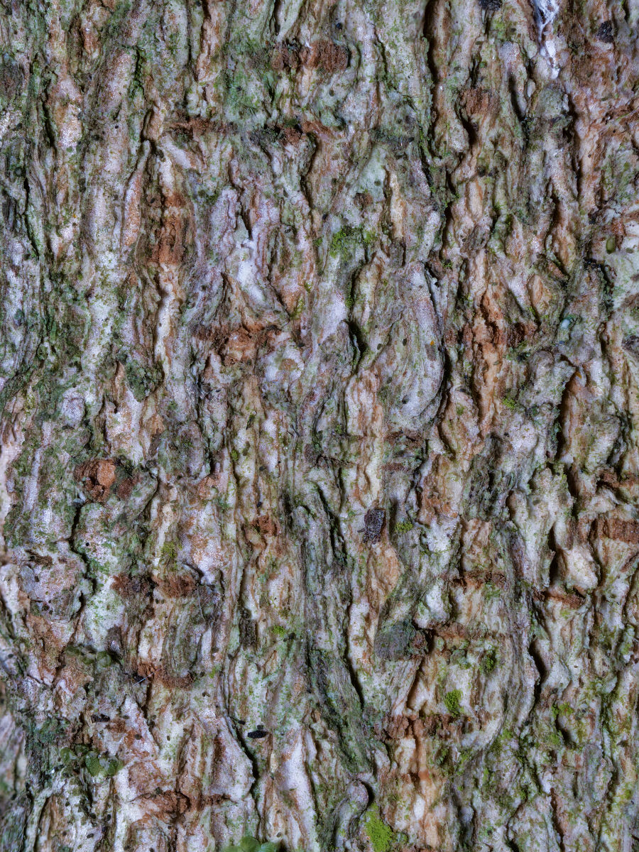
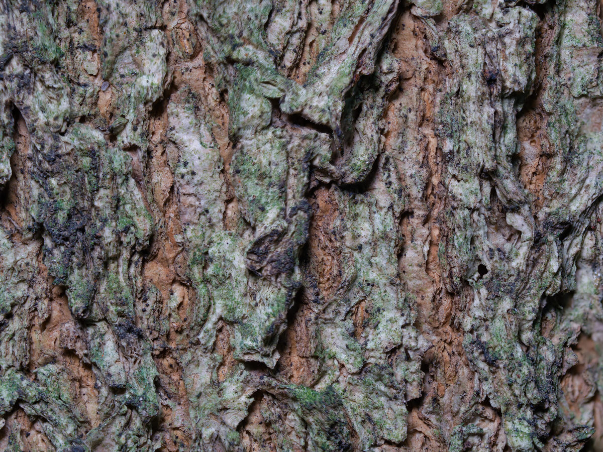
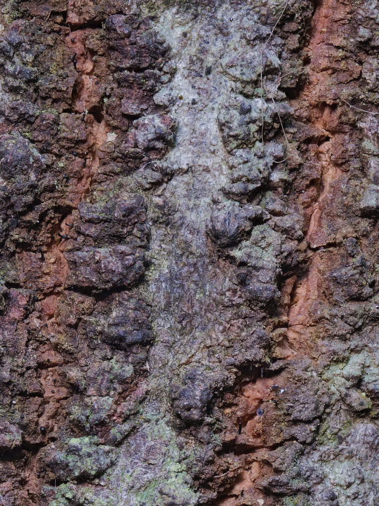
Tree barks are polymorphic, which means their colours and textures vary greatly. As fingerprints are for human’s, barks are for trees, unique. It is a key reason trees are rarely identified by their bark, but mainly by their leaves, flowers, fruits or seeds.

I wanted to describe my bark macro images with more objectivity for the Atlas of Living Australia (ALA). I set about trying to work out a way where I could broadly describe a bark’s colours and textures. I was not trying to be definitive or scientifically exact, but objective, descriptive and accurate. Simplicity would be a plus.

Bark’s age and type

A tree’s bark is influenced by many factors, but age is important. Wherever possible, I try and work out a tree’s age. My three broad categories are:

1. Young;
2. Mature; and
3. Old.

A barks colour and texture can vary greatly between the three ages.

When describing bark, I also try and work out whether the bark is initial periderm or active periderm (which can vary between young, mature and old trees). Generally, the resulting colour palette is a mixture of initial periderm (older/outer bark), the active periderm (young/inner bark) and any colour contamination caused by mosses, lichens or sap.

Whether the bark is initial periderm or active periderm is also important, but this will be discussed in Part 2 on textures.

Describing colour

Macro image creation

The colour palette is influenced by the way my macro images are created. Most of my images are created using this process:

1. evenly light the bark, using an LED light set at daylight temp (5300 Kelvin) (and some using a flash for non stacked images);
2. focus stack the image, using a feature known as Post Focus on a Panasonic camera;
3. use a flat colour profile (CineD) in camera to maximise the capture of colours;
4. post process images with a simple curves adjustment (or use PhotoLemur 3) to achieve a good range of colours, while keeping colours realistic;
5. sharpen the image to remove artefacts caused by stacking (using Topaz Sharpen AI). Mostly movement artefacts, as my images are nearly all taken in the field; and
6. reduce image in size to 2560 pixels on its long side. Most images are 2-3 meg is size at the end of the process when uploaded to the ALA. I do retain master files which are much larger, over 20 megs up to 120 megs.

My processed images look more colourful than the brown/grey hues seen in the usual photos taken of the whole trunk, due to careful lighting, correct exposure and processing. The images reveal what is really there if you look closely. Most images are 2X or 2.5X in magnification, so you can see much more detail, than you can with your eye looking at the bark in real life. The images show an area of bark roughly the size of a postage stamp! (Although more recently I have been add wider shots as well) . The exact area varies depending on the lens used and composition.

I am also trying to add the year the tree was planted and/or its height. I am using an iPhone app to get the tree height in the field called Arboreal. Android version also available.

Using the RGB colour palette

Computers use an RGB colour palette. It is additive palette made up of one or more of Red, Green or Blue colours (hence RGB).

The ALA images are mostly viewed on computer, tablet or phone screens. It made sense to use the RGB colour palette for my colour descriptions.

RGB colour palettes are commonly described by decimal values, hexadecimal values or names. I prefer colour names to their Hex code (#FFEBCD) or RGB decimal code (255, 235, 205). Otherwise known as Blanched Almond.

I looked for a way to choose a source image, broadly representing the bark type, and then create a colour palette identifying the ten most dominant hues (colours). If a species has considerable variation in its bark and I have enough samples, I will create a bark montage, trying to get a broader colour palette of the species.

The result for Owenia cepiodora (Onion Cedar) is:

Colour description using the screenshots

Using the ten dominant colours screenshot we can see the bark’s main hues are dark browns, grey and some red-browns. There are four brown hues, four grey hues and two red-brown hues including Bistre, Olive Drab, Taupe Grey, Dark Grey and Rosy Brown.

The palette not only tells you the names of the ten main colours, but more importantly is a visual guide to the main hues/colours in the image.

Why does the colour palette look slightly different to the image? In the colour palette you see each distinct colour, but the image is a mixture of these colours and many more. It is like looking at an artist’s various paint colours, before the colours are mixed on their palette and put on the canvas. The palette is just identifying the ten main colours used by nature, not how nature mixes all the colours.

The choice proved visually appealing, but also informative. I noticed colours in the palette not immediately obvious when I looked directly at the image. It improved my objectivity.

Colour’s complexity

Colours are very complex so I investigated other ways to use colour and reveal more information about an image, without undue complexity. I found an ImageJ2 plug-in (Fiji Distribution), called Color Inspector 3D. It allowed me to quickly identify all the colours and tonality in the image and reduce that complexity to a smaller list of core colours and tones, without materially changing the look of the image, using histogram mode to give the core colours. Using our source image, it yields this information: Colour Palette: RGB. Number of pixels: 786,432. All colours present: 133,130. Histogram core colours: 162.

RGB All colors screenshot

RGB Histogram screenshot

Color Inspector 3D shows the colours based not only on the Red, Green and Blue channels (see R, G and B on the screenshot), but also 256 shades of tonality. Darks (Blacks) on the bottom left (see 0) and Whites (Highlights) in the opposite corner which would be 255. There are 256 tones, as 0 is the first tone counted (255+1=256).

On our sample image, the plug-in can reduce the colours from 133,130 down to 162 with no obvious visual change to the image (occasionally some images do show a small change). Color Inspector 3D is only displaying 162 colours in the RGB Histogram screenshot. The eye and brain cannot discern the full 133,130 colours in the RGB All Colors screenshot, they need only 162.

Color Inspector 3D, in Histogram mode, allows you to export a LUT file setting out the colours and their frequency displaying in the Histogram. The LUT file for the 162 core colours is here. The LUT file, in csv format, gives the values for the red, green and blue channels making up the 162 core colours listed.

The plug-in allows you to rotate the colour square on the right in real time to better explore the relationship between the Red, Green, Blue channels and the tonality.

If the full range of screenshots are added to ALA, you see the source image (sometimes with a scale added), the colour palette of the ten dominant colours, then RGB All Colors screenshot followed by the core colours in the RGB Histogram screenshot. These last two screenshots are produced in Color Inspector 3D plug-in. These palettes allow a quick comparison and a deeper dive into the bark’s complex colour palette, than the ten dominant colours can. The viewer can make their own observations.

This approach has shown how lacking some descriptions of bark colours are. I have seen examples where the dominant hue is not even mentioned (which could also be caused by bark variation). Instead of making subjective comments about colours, this approach is more objective, visual and descriptive, thanks to the computer.

Hue, saturation, lightness (HSL)

When processing images it is common to make Hue, Saturation and Lightness adjustments (HSL). Hue is what colour, saturation is how much colour and lightness is the brightness of the colour (or its tonality from light (white) to dark (black)). Screenshots of HSL All Colors and HSL Histograms are also supplied using HSL. It gives more insight into the colour palette than RGB alone, like this:

HSL All Colors screenshot

HSL Histogram screenshot

Colour description using the screenshots

Using the ten dominant colours screenshot we can see the bark’s main hues are dark browns, grey and some red-browns. There are four brown hues, four grey hues and two red-brown hues including Bistre, Olive Drab, Taupe Grey, Dark Grey and Rosy Brown.

Looking at the 162 core colours, they are in the midtones with some darker brown hues but minimal grey highlights (the two Histogram screenshots). Both All Colors screenshots confirm this.

Some darker brown hues are heavily saturated, while a few grey hues reach up into the highlights (HSL Histogram screenshot).

Word of warning

I am using the palettes as a visual guide. The total number of colours could be overstated in some images, because the software may read, for example, the shadow areas in the image as darker colours, when in fact they would be more akin to the main colours. I place more emphasis on the ten dominant colours and the core colours, than the total number of colours. Warning: using the sRGB colour palette, instead of the AdobeRGB palette, can also increase the number of core colours in the same image (at least in the tests I did).

Colour managed computers

Most computers are not calibrated to correctly display colours. My images are processed on a professional grade, calibrated colour monitor.

One advantage of my approach is the source image and the colour palettes will display consistently wrong on any uncalibrated monitor (between the images in a set).

PART 2 – DESCRIBING TEXTURE

I was thinking about a document where the key characteristics of the bark (flower or leaf), both colour and texture could be summerised and described. Again the objective was for the descrition to be objective, descriptive and accurate The document goes with the various screenshots posted in Part 1. There are three parts to the document

1. General description

Here I describe the scientific name, common names, the tree’s age and height (if known). If the image is bark, I also describe the periderm, which is mainly initial periderm (older/outer bark) or active periderm (young/inner bark).

2. Color description

The colour information is extracted from the screen captures from Color Inspector 3D, discussed in Part 1. It covers pixels numbers, total colours, core colours and other relevant information.

3. Texture description

This part describes attributes of the bark based on 18 categories. A visual guide is provided, with a discussion of lenticels, ridges, furrows, scales and plates. The 18 categories are based on those described in Tree Bark: A Color Guide, Hugues Vaucher, 2003. The additional discussion of lenticels, ridges, furrows, scales and plates is based on Bark: A Field Guide to Trees of the Northeast, Michael Wojtech, 2011.

It makes sense when you look at a sample document, here Owenia cepiodora.